Watt curve: Difference between revisions
From JSXGraph Wiki
mNo edit summary |
A WASSERMANN (talk | contribs) No edit summary |
||
| (6 intermediate revisions by 2 users not shown) | |||
| Line 1: | Line 1: | ||
=Trace= | |||
With JSXGraph elements can be traced to visualize construced loci. | With JSXGraph elements can be traced to visualize construced loci. | ||
<html> | <html> | ||
<input type="button" value="Clear trace" onClick="clearTrace()" /> | <input type="button" value="Clear trace" onClick="clearTrace()" /> | ||
< | </html> | ||
board = JXG.JSXGraph.initBoard('jxgbox', { | <jsxgraph box="jxgbox" width="600" height="450"> | ||
board = JXG.JSXGraph.initBoard('jxgbox', {boundingbox: [-2, 16, 22, -2], axis: true, grid: false}); | |||
p1 = board.create('point', [7, 8], {face:'x',size:4,name:"",fixed:true}); | |||
p1 = board. | p2 = board.create('point', [15, 8], {face:'x',size:4,name:"",fixed:true}); | ||
p2 = board. | c1 = board.create('circle', [p1, 4.5]); | ||
c1 = board. | c2 = board.create('circle', [p2, 4.5]); | ||
c2 = board. | g1 = board.create('glider', [0, 0, c1], {size:3,name:"Drag me"}); | ||
g1 = board. | c3 = board.create('circle', [g1, 8]); | ||
c3 = board. | g2 = board.create('intersection', [c2,c3,0], {size:3, name: ""}); | ||
g2 = board. | g3 = board.create('intersection', [c2,c3,1], {size:3, name: ""}); | ||
g3 = board. | m1 = board.create('midpoint', [g1,g2], {face:'[]',size:3,withLabel:false,trace:true}); | ||
m1 = board. | m2 = board.create('midpoint', [g1,g3], {face:'[]',size:3,withLabel:false,trace:true,strokeColor:'green'}); | ||
m2 = board. | |||
function clearTrace() { | function clearTrace() { | ||
| Line 26: | Line 23: | ||
m2.clearTrace(); | m2.clearTrace(); | ||
} | } | ||
</ | </jsxgraph> | ||
==References== | ==References== | ||
* [http://en.wikipedia.org/wiki/Watt_curve] | * [http://en.wikipedia.org/wiki/Watt_curve http://en.wikipedia.org/wiki/Watt_curve] | ||
==The underlying JavaScript code== | ==The underlying JavaScript code== | ||
<source lang="javascript"> | <source lang="javascript"> | ||
board = JXG.JSXGraph.initBoard('jxgbox', { | board = JXG.JSXGraph.initBoard('jxgbox', {boundingbox: [-2, 16, 22, -2], axis: true, grid: false}); | ||
p1 = board.create('point', [7, 8], {face:'x',size:4,name:"",fixed:true}); | |||
p2 = board.create('point', [15, 8], {face:'x',size:4,name:"",fixed:true}); | |||
p1 = board. | c1 = board.create('circle', [p1, 4.5]); | ||
p2 = board. | c2 = board.create('circle', [p2, 4.5]); | ||
c1 = board. | g1 = board.create('glider', [0, 0, c1], {size:3,name:"Drag me"}); | ||
c2 = board. | c3 = board.create('circle', [g1, 8]); | ||
g1 = board. | g2 = board.create('point', [board.intersectionFunc(c2,c3,0)], {size:3, name: ""}); | ||
c3 = board. | g3 = board.create('point', [board.intersectionFunc(c2,c3,1)], {size:3, name: ""}); | ||
g2 = board. | m1 = board.create('midpoint', [g1,g2], {face:'[]',size:3,withLabel:false,trace:true}); | ||
g3 = board. | m2 = board.create('midpoint', [g1,g3], {face:'[]',size:3,withLabel:false,trace:true,strokeColor:'green'}); | ||
m1 = board. | |||
m2 = board. | |||
function clearTrace() { | function clearTrace() { | ||
| Line 54: | Line 48: | ||
m2.clearTrace(); | m2.clearTrace(); | ||
} | } | ||
</source> | |||
=Compute Locus Equation= | |||
One way to compute the locus equation of the traced points in the above construction is the Groebner-Basis-Method. Applying this method to the above construction we get this polynomial: | |||
<math>16e^4s^2 - 96e^3s^3 + 208e^2s^4 - 192es^5 + 64s^6 + 16e^4t^2 - 96e^3st^2 + 288e^2s^2t^2 - 384es^3t^2 + 192s^4t^2 + 80e^2t^4 - 192est^4 + 192s^2t^4 + 64t^6 + 136e^3s - 680e^2s^2 + 1088es^3 - 544s^4 - 1432e^2t^2 + 1088est^2 - 1088s^2t^2 - 544t^4 + 289e^2 - 1156es + 1156s^2 + 1156t^2</math> | |||
Where in this case <math>e=8</math>. Setting the polynomial to zero and plotting that equation with Maple results the following picture. | |||
[[Image:Plot_watt_curve.jpeg]] | |||
[[Category:Examples]] | [[Category:Examples]] | ||
[[Category:Curves]] | [[Category:Curves]] | ||
Latest revision as of 16:17, 20 February 2013
Trace
With JSXGraph elements can be traced to visualize construced loci.
References
The underlying JavaScript code
board = JXG.JSXGraph.initBoard('jxgbox', {boundingbox: [-2, 16, 22, -2], axis: true, grid: false});
p1 = board.create('point', [7, 8], {face:'x',size:4,name:"",fixed:true});
p2 = board.create('point', [15, 8], {face:'x',size:4,name:"",fixed:true});
c1 = board.create('circle', [p1, 4.5]);
c2 = board.create('circle', [p2, 4.5]);
g1 = board.create('glider', [0, 0, c1], {size:3,name:"Drag me"});
c3 = board.create('circle', [g1, 8]);
g2 = board.create('point', [board.intersectionFunc(c2,c3,0)], {size:3, name: ""});
g3 = board.create('point', [board.intersectionFunc(c2,c3,1)], {size:3, name: ""});
m1 = board.create('midpoint', [g1,g2], {face:'[]',size:3,withLabel:false,trace:true});
m2 = board.create('midpoint', [g1,g3], {face:'[]',size:3,withLabel:false,trace:true,strokeColor:'green'});

function clearTrace() {
    m1.clearTrace();
    m2.clearTrace();
}
Compute Locus Equation
One way to compute the locus equation of the traced points in the above construction is the Groebner-Basis-Method. Applying this method to the above construction we get this polynomial:
[math]\displaystyle{ 16e^4s^2 - 96e^3s^3 + 208e^2s^4 - 192es^5 + 64s^6 + 16e^4t^2 - 96e^3st^2 + 288e^2s^2t^2 - 384es^3t^2 + 192s^4t^2 + 80e^2t^4 - 192est^4 + 192s^2t^4 + 64t^6 + 136e^3s - 680e^2s^2 + 1088es^3 - 544s^4 - 1432e^2t^2 + 1088est^2 - 1088s^2t^2 - 544t^4 + 289e^2 - 1156es + 1156s^2 + 1156t^2 }[/math]
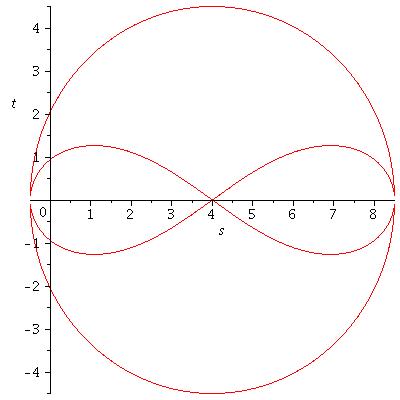
Where in this case [math]\displaystyle{ e=8 }[/math]. Setting the polynomial to zero and plotting that equation with Maple results the following picture.
